Tuesday, June 28, 2016

Sparse voxel octree meshing

I have started experimenting with a blocky voxel renderer à la Minecraft. This post describes and compares algorithms to go from a voxel representation to a triangle mesh. I take some terminology from this great blog article where the author introduces three meshing algorithms: stupid, naive and greedy. The “stupid” algorithm generates six faces for every filled voxel. The “naive” meshing algorithm culls faces that cannot be seen because they are between two filled voxels. The “greedy” meshing algorithm merges faces to further reduce their number.

The same author has also written another blog post that compares different voxel representations. I agree with this blog post’s claim that for a voxel representation iteration is more important than random access. But I disagree that octrees are bad for iteration. Iterating through an octree touches every node exactly once and is therefore linear in the number of leafs.

We will compare the “stupid” and “naive” meshing algorithms on a static grid representation and an octree representation.

Octrees

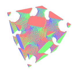
The number of leafs in an octree is much lower than the number of voxels in a grid. Consider the following two voxel scenes:

Ball with resolution 64 Trigonometric function with resolution 64

The left is a ball of resolution 64^3 and the right is a 64^3 sampled trigonometric function taken from here.

The following table shows the number of voxels in a grid versus the number of leafs in an octree for different resolutions. The number of voxels is independent of the scene. The number of leafs is shown for the two example scenes above.

Resolution Voxels Leafs/Ball Leafs/Function
8 512 232 225
16 4,096 1,408 1,443
32 32,768 5,944 6,924
64 262,144 24,760 33,860
128 2,097,152 98,848 140,260
256 16,777,216 408,808 560,148

The number of voxels is way higher than the number of leafs, especially as the resolution grows. This is not only a waste of space but also of time. If you want to iterate through a grid you have to touch every single voxel. But with octrees you can run through its leafs and never look at individual voxels.

Octree definition

We will work with the following definition of an octree:

data Octree a =
  Full a |
  Children (Oct (Octree a))

data Oct a = Oct a a a a a a a a

An Octree a is either full and carries a value of type a or it has children. The children are held in an Oct. An Oct a is an 8-tuple of values of type a. For example this octree is subdivided once and has eight children filled with different letters:

exampleOctree :: Octree Char
exampleOctree = Children (Oct
  (Full 'a') (Full 'b') (Full 'a') (Full 'a')
  (Full 'c') (Full 'a') (Full 'a') (Full 'c'))

We will have to enumerate all values in an octree. The enumerate function takes an octree and produces a list of all its leaf values.

enumerate :: Octree a -> [a]
enumerate (Full a) =
  [a]
enumerate (Children children) =
  concatMap enumerate (octToList children)

octToList :: Oct a -> [a]
octToList (Oct a0 a1 a2 a3 a4 a5 a6 a7) =
  [a0, a1, a2, a3, a4, a5, a6, a7]

If we have a full octree we produce the value in a singleton list. If the given octree has children we recursively enumerate all children and concatenate the results.

Paths

We will also need to know where an octree’s leafs are located in space. We can uniquely identify a node in an octree with its path from the root. We introduce a Path data type (sometimes called locational code):

data Path = Path Resolution Location
type Resolution = Int
type Location = V3 Int

A path consists of four numbers: its resolution and its location’s three coordinates.

In the following image you can see quads with their corresponding quadtree paths:

Quadtree paths

In a quadtree a path consists of only three numbers: a resolution and two coordinates.

We will have to annotate each leaf in an octree with its path:

annotatePath :: Path -> Octree a -> Octree (Path, a)
annotatePath path (Full a) =
  Full (path, a)
annotatePath path (Children children) =
  Children (zipOctWith annotatePath (childPaths path) children)

Again we have two cases. If the given octree is completely filled with a value a we return the given path paired with this value. If the given octree is subdivided we recursively annotate all its children. We zip the children with an Oct Path containing the immediate children’s paths.

Cubes

Every octree path denotes a 3D cube. A cube consists of a size and a position.

data Cube = Cube Float (V3 Float)

We get the cube corresponding to a path with the pathCube function:

pathCube :: Path -> Cube
pathCube (Path resolution location) =
  Cube size position where
    size = recip (realToFrac resolution)
    position = size *^ fmap realToFrac location

The size of the cube is the reciprocal resolution (as a Float) and the position is the location scaled by the size. For example the path Path 4 (V3 1 0 0) corresponds to the cube Cube 0.25 (V3 0.25 0 0).

With these definitions we can start meshing.

Meshing

We are going to work with the following block type:

data Block = Air | Solid

A block is either filled with air or it is solid.

A mesh is a list of faces. A face is a 3D quad that has a position and is spanned by two vectors.

data Face = Face (V3 Float) (V3 Float) (V3 Float)

Our meshing functions will have type Octree Block -> [Face]. They will take an octree of blocks and produce a list of faces.

Stupid octree meshing

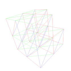
“Stupid meshing” is a technical term that means we generate six faces for every solid voxel. This results in lot’s of faces that can never be seen because they are hidden by other solid blocks. Here is a screenshot:

Octree missing corner Interior triangles

On the left you see a very simple voxel scene. On the right you see the same scene in wireframe mode.

Ok, now let’s implement stupid meshing for octrees:

stupidMesh :: Octree Block -> [Face]
stupidMesh octree =
  concatMap leafFaces (enumerate (annotatePath rootPath octree))

leafFaces :: (Path, Block) -> [Face]
leafFaces (_, Air) =
  []
leafFaces (path, Solid) =
  cubeFaces (pathCube path)

The stupid meshing algorithm enumerates all leafs in the octree annotated with their paths. It applys the leafFaces function to each annotated leaf and concatenates the results.

The leafFaces function takes a pair of a path and a block and returns a list of faces. If the block type is Air we generate an empty list of faces. If the block type is Solid we generate the list of six faces of the cube corresponding to the path.

Later we’ll compare this meshing algorithm’s performace to others.

Naive octree meshing

“Naive meshing” means that we generate a face only when a solid block is adjacent to a transparent one. In other words: no inside faces. Here are two screenshots:

Inside a solid sphere Inside a solid wireframe sphere

They are taken from inside of a completely solid sphere. Triangles are only generated where a solid block touches an air block.

The essence of the algorithm is the neighbour function. Given an octree and its direct neighbour in positive X direction it annotates every value in the given octree with its neighbour’s value.

neighbour :: Octree a -> Octree a -> Octree (a, a)
neighbour (Full value) (Full neighbourValue) =
  Full (value, neighbourValue)
neighbour (Full value) (Children neighbourChildren) =
  neighbour
    (Children (homogeneousOct (Full value)))
    (Children neighbourChildren)
neighbour (Children children) (Full neighbourValue) =
  neighbour
    (Children children)
    (Children (homogeneousOct (Full neighbourValue)))
neighbour (Children children) (Children neighbourChildren) =
  Children (zipOctWith neighbour children newNeighbours) where
    (Oct _ c1 _ c3 _ c5 _ c7) = children
    (Oct n0 _ n2 _ n4 _ n6 _) = neighbourChildren
    newNeighbours = Oct c1 n0 c3 n2 c5 n4 c7 n6

We have to consider four cases. In the base case both octrees are completely filled. We just pair up their values.

We reduce the cases where one given octree is full and the other one has children to the fourth case where both octrees have children.

In the fourth case where both octrees have children we recurse. We have to be careful to pick the correct neighbours for the recursive calls. The following picture illustrates the idea with quadtrees:

Quadtree neighbours

The top two quadtrees depict the arguments and the bottom quadtree depicts the recursive calls. For example we recurse into the lower left quad with arguments c0 and c1.

Now that we know how to annotate an octree with neighbouring information, naive meshing for the positive X direction is:

naiveMeshPositiveX :: Octree Block -> [Face]
naiveMeshPositiveX octree =
  mapMaybe neighbourFacePositiveX (
    enumerate (annotate rootPath (
      neighbour octree)))

neighbourFacePositiveX :: (Path, (Block, Block)) -> Maybe Face
neighbourFacePositiveX (path, (Solid, Air)) =
  Just (cubeFacePositiveX (pathCube path))
neighbourFacePositiveX _ =
  Nothing

The naiveMeshPositiveX function enumerates all octree leafs annotated with their path and their neighbour’s value. It calls the neighbourFacePositiveX function on each annotated leaf and gathers up the results.

The neighbourFacePositiveX function takes a path paired with a pair of blocks. If the first block is solid and the second block is air we return a face for the cube that corresponds to the path. If not we return Nothing.

This only generates faces in the positive X direction. To generate faces for the other directions we have to mirror and transpose the octree before and after annotating each leaf’s neighbour and generate the cubes’ corresponding faces.

Benchmarks

The following table shows the number of faces for the ball scene generated by different algorithms for different resolutions:

Resolution Grid/stupid Octree/stupid Grid/naive Octree/naive
8 816 480 192 192
16 9,408 3,360 984 984
32 87,552 15,648 4,344 4,056
64 759,312 68,496 18,288 17,064
128 6,324,768 295,584 75,192 70,872
256 51,648,096 1,201,392 304,608 287,616

Naive meshing generates much fewer faces than stupid meshing.

The following table shows the time taken to produce the mesh for the ball with different resolutions. The time is in milliseconds.

Resolution Grid/stupid Octree/stupid Grid/naive Octree/naive
8 0.187 0.010 0.220 0.004
16 1.973 0.119 2.308 0.022
32 16.870 1.066 21.090 0.224
64 136.000 4.847 164.200 1.349
128 1154.000 20.930 1288.000 5.547
256 9186.000 85.760 10740.000 22.350

Meshing an octree is much faster than meshing a grid.

Thank you for reading the whole post. Comments are more than welcome!

Monday, February 15, 2016

Fixing a space leak by copying thunks.

After my last blog post about FRP I got feedback that my approach makes it easy to accidentally introduce space leaks. I also got helpful pointers to resources. In this post I give an example program with a space leak and discuss how to fix it.

The Behavior type

We work with the following Behavior type:

data Behavior next a =
  AndThen a (next (Behavior next a))

now :: Behavior next a -> a
now (AndThen a _) = a

future :: Behavior next a -> next (Behavior next a)
future (AndThen _ nextBehavior) = nextBehavior

A behavior is a stream of values. It has a current value that we can extract with now and a future behavior that we can extract with future. The Behavior type constructor has two type parameters. The first type parameter called next lets us decide which effects we want to allow when we advance to the next iteration. The second type parameter called a is the type of values this behavior carries. The behavior type is the same (up to renaming) as Cofree.

We can instantiate next with different types. We have instances of Functor and Applicative for Behavior as long as we instantiate next with types that have instances of Functor and Applicative:

instance (Functor next) => Functor (Behavior next) where

  fmap f (a `AndThen` nextAs) =
    (f a) `AndThen` (fmap (fmap f) nextAs)


instance (Applicative next) => Applicative (Behavior next) where

  pure a = a `AndThen` (pure (pure a))

  (f `AndThen` nextFs) <*> (x `AndThen` nextXs) =
    (f x) `AndThen` (liftA2 (<*>) nextFs nextXs)

Just a note: this Applicative instance is different to the one for Cofree.

In the last post next was IO which allows arbitrary side-effects and is hard to reason about. But we can for example instantiate next to Identity which means we get ordinary pure lists. Because behaviors over Identity are like lists we have correspondences between fmap and map, now and head and liftA2 and zipWith.

To test behaviors where next is Identity we use a function that writes its elements to the console:

runList :: (Show a) => Behavior Identity a -> IO ()
runList (a `AndThen` as) = do
  print a
  runList (runIdentity as)

We use runIdentity to get the next behavior to run.

A leaky program

Let’s create a program with a space leak! We will take inspiration from programs on lists. We use two functions that correspond to enumFrom and repeat called countFrom and always. countFrom takes an Int and starts counting from that number. always lets us transport any value indefinitely far into the future. They work for behaviors with all sorts of instantiations for next as long as they are Applicative because they use pure.

countFrom :: (Applicative next) => Int -> Behavior next Int
countFrom i = i `AndThen` pure (countFrom (i + 1))

always :: (Applicative next) => a -> Behavior next a
always a = a `AndThen` pure (always a)

We will use countFrom to create a behavior called numbers. We will pair it with a behavior that is always zero. When we run the final program (for historical reasons named animations) the output looks like this:

> animations
(0,0)
(1,0)
(2,0)
(3,0)
...

The trick is that the second element of the printed pairs will require a reference to numbers. This means that numbers cannot be garbage collected. As numbers expands it will take up more and more heap space. The program looks like this:

main :: IO ()
main = do

  let numbers = countFrom 0

  let alwaysNumbers = fmap now (always numbers)

  let pairs = liftA2 (,) numbers alwaysNumbers

  runList pairs

We transport numbers into the future using always. This would be a behavior of behaviors. At each point in time we extract the current value to get a behavior of Int using fmap now. We call the resulting behavior alwaysNumbers. Then we zip numbers and alwaysNumbers together using liftA2. Finally we run the behavior (which means to keep iterating and printing).

Here is a heap profile created by invoking the program with animations +RTS -h. We invoked hp2pretty on animations.hp to produce the following picture:

list heap profile

Space usage grows linearly with time.

The problem pictorially

The following shows a sketch of the heap after the program printed (3,0):

list heap sketch

The chain of cells represents the numbers value. The two arrows coming from the top are two references: one to the original numbers value and one to the current element. The little cloud represents the unevaluated thunk that is the future behavior.

Now, what if we didn’t have a single chain of cells? What if we copied all future behavior thunks and did not replace them? We would get a picture like this:

copying heap sketch

The garbage collector will reclaim the cells for 1 and 2 because there are no references to them.

Copying thunks

Let me demonstrate what I mean with “copying thunks” with a small ghci session. On a high level we bind exampleThunk to the pure value True and evaluate it three times. To observe the evaluation we use trace from Debug.Trace to print "thunk evaluated" upon evaluation.

> import Debug.Trace
> let exampleThunk = trace "thunk evaluated" True
> exampleThunk
thunk evaluated
True
> exampleThunk
True
> exampleThunk
True

The string "thunk evaluated" appears only once. Later evaluations reuse the previously computed value. Usually this is a good thing because the thunk might have been costly to evaluate.

But now what we’d like to have are two functions with the following signatures:

copy :: a -> Copy a
getCopy :: Copy a -> a

This time we use functions copy and getCopy to make the evaluation of exampleThunk happen multiple times.

> import Debug.Trace
> let exampleThunk = trace "thunk evaluated" True
> let copyOfExampleThunk = copy exampleThunk
> getCopy copyOfExampleThunk
thunk evaluated
True
> getCopy copyOfExampleThunk
thunk evaluated
True
> getCopy copyOfExampleThunk
thunk evaluated
True

Whenever we force the result of getCopy the thunk is evaluated. We do not replace the original thunk by the result.

The Copy Applicative

I don’t think it is possible to get the desired behavior of Copy with current GHC. But luckily Joachim Breitner has published an experiment in the form of the ghc-dup package a few years ago. It works (as a prototype) for GHC 7.4 and GHC 7.6. It provides a function dup that allows us to create the desired Copy type and make it an Applicative:

data Copy a = Copy a

copy :: a -> Copy a
copy a = Copy a

getCopy :: Copy a -> a
getCopy (Copy a) = case dup a of Box a' -> a'

instance Functor Copy where
  fmap f a = copy (f (getCopy a))

instance Applicative Copy where
  pure a = copy a
  f <*> a = copy ((getCopy f) (getCopy a))

We are careful to never directly use the thunk inside Copy. Instead we copy it with getCopy.

Heap profile with copying

Now we can instantiate our behavior with Copy instead of with Identity and still run it like so:

runCopying :: (Show a) => Behavior Copy a -> IO ()
runCopying (a `AndThen` copyAs) = do
  print a
  runCopying (getCopy copyAs)

We use getCopy instead of runIdentity to get the next behavior. This allows us to change the previously leaky program to use Copy instead of Identity by using runCopying instead of runList:

main :: IO ()
main = do

  let numbers = countFrom 0

  let alwaysNumbers = fmap now (always numbers)

  let pairs = liftA2 (,) numbers alwaysNumbers

  runCopying pairs

We get the same output but the following heap profile:

enter image description here

The space leak is gone.

Conclusion

GHC uses call-by-need by default. It allows for call-by-value via seq and deepseq. Sometimes we want call-by-name. I believe that if ghc-dup was a feature supported by GHC we would see it used.

Wednesday, January 13, 2016

FRP for free

The connection between functional reactive programming and temporal logic is well known and studied. I want to describe how an FRP interface in Haskell based on temporal logic could look like. I should also cite these slides from Uni Muenchen and this paper.

Inspiration from temporal logic

If we go to wikipedia we see that temporal logic has three basic unary operators called Next, Globally and Finally (abbreviated X, G and F). They are explained further down on that page. Globally and Finally translate to the familiar Behavior and Event types. Next is a type I have never seen in an FRP library before. It protects the future from access in the now, similar to MomentIO or Now.

In the equivalences section under Special temporal properties we see two interesting equivalences that we take to be our basic axioms:

G Φ ≡ Φ ∧ X(G Φ)
F Φ ≡ Φ ∨ X(F Φ)

Translated to Haskell this is

data Behavior a = AndThen {
  now :: a,
  future :: Next (Behavior a) }

data Event a =
  Occured a |
  Later (Next (Event a))

Behavior is Cofree instantiated with Next and Event is Free instantiated with Next.

We have to make one other assumption: that Next is an instance of Applicative. In this post for simplicity we define Next to be IO:

type Next = IO

Deriving temporal logic axioms

My search did not reveal what axioms temporal logic usually rests on. But temporal logic is a specific modal logic and as far as I understand modal logic axioms sometimes include (notation taken from wikipedia and explained below):

  • N: p → □p
  • K: □(p → q) → (□p → □q).
  • T: □p → p
  • 4: □p → □□p
  • B: p → □◇p
  • D: □p → ◇p
  • 5: ◇p → ◇□p

Ok, this notation is different to what we saw earlier. The little box is what we called G and corresponds to Behavior and the little diamond is what we called F and corresponds to Event. Under this notation X (called Next in our interpretation) would be denoted with a little circle.

Axioms N and K are found in all modal logics while the others are more optional. N is called the Necessitation Rule, axiom K is called the Distribution Axiom and axiom T is called the Reflexivity Axiom. In Haskell they correspond to pure, ap and extract. Axiom 4 has no long name in logic but in Haskell it is called duplicate.

These axioms become theorems because they follow from our basic axioms. We can derive them using our basic axioms which is to say we can implement them using our data type definitions. For example a Behavior that is always the same is:

always :: a -> Behavior a
always a = a `AndThen` pure (always a)

This corresponds to the N axiom. Implementations of some of the other axioms seem trivial and do not make sense as general purpose combinators.

Implementing FRP functions

On the other hand we can easily implement functions known from FRP libraries. For example an event that never happens:

never :: Event a
never = Later (pure never)

Or we can sample a behavior when an event occurs:

sample :: Event a -> Behavior b -> Event (a, b)
sample (Occured a) (AndThen b _) =
  Occured (a, b)
sample (Later nextEvent) (AndThen _ nextBehavior) =
  Later (liftA2 sample nextEvent nextBehavior)

A symmetric IO interface

If we have the ability to lift IO actions into Next we get a nice, symmetric IO interface similar to fromPoll, reactimate and planNow:

plan :: Event (Next a) -> Next (Event a)
plan (Occured next) =
  fmap Occured next
plan (Later next) =
  fmap (Later . plan) next

poll :: Behavior (Next a) -> Next (Behavior a)
poll behavior =
  liftA2 AndThen
    (now behavior)
    (fmap poll (future behavior))

Luckily in our case Next is IO and we can lift IO actions into Next with:

syncIO :: IO a -> Next a
syncIO = id

To poll the current time using getCurrentTime we would write the following:

currentTime :: Next (Behavior UTCTime)
currentTime =
  poll (always (syncIO getCurrentTime))

We get an event that fires upon the next user input with:

nextLine :: Next (Event String)
nextLine =
  plan (Occured (syncIO getLine))

Running Behaviors and Events

We can run an event until it occurs, performing all side effects while doing so:

runNext :: Next a -> IO a
runNext = id

runEvent :: Event a -> IO a
runEvent event = case event of
  Occured a ->
    return a
  Later nextEvent -> do
    event' <- runNext nextEvent
    runEvent event'

An example application

Let’s finish with a small example application. It will keep asking the user for input, then print the user’s input and the current time. It will stop if the user enters "exit". The parameters of this function are the event of the next user input and a behavior that carries the current time.

loop :: Event String -> Behavior UTCTime -> Event ()

loop (Occured "exit") _ = do
  Occured ()

loop (Occured message) (AndThen time futureTime) =
  Later (
    syncIO (putStrLn (show time ++ ": " ++ message)) *>
    liftA2 loop nextLine futureTime)

loop (Later nextEvent) (AndThen _ futureTime) =
  Later (
    liftA2 loop nextEvent futureTime)

And finally we run this loop:

main :: IO ()
main = runEvent (Later (
  liftA2 loop nextLine currentTime))

Example interaction:

> hi
2016-01-13 11:44:58.059605 UTC: hi
> what's new
2016-01-13 11:45:00.178503 UTC: what's new
> exit

In conclusion we have taken two temporal logic theorems as axioms and based an implementation of FRP on them. This implementation happens to be Cofree for behaviors and Free for events over a Next functor. In this post we used IO for Next but I have a feeling that the power of this approach lies in the fact that we can vary this functor.